A manifestation of order and beauty in nature is called symmetry.
The search for fundamental symmetries is the primary goal of physics.
Only in this way can we unveil the workings of the universe, from its beginning to its possible end.
Curriculum Vitae
Education
Ph.D. in Theoretical Physics at TU München
Munich, Germany
Advisor: Dr. Danny van Dyk
Title: "Applications of Light-Cone Sum Rules in Flavour Physics"
2017 - 2020
Master's Degree in Physics at Università "La Sapienza"
Rome, Italy
Grade: 110/110 with honours
2014 - 2016
Bachelor's Degree in Physics at Università degli Studi di Perugia
Perugia, Italy
Grade: 110/110 with honours
2011 - 2014
Academic Positions
Emmy Noether Group Leader at University of Bonn
Helmholtz-Institut für Strahlen- und Kernphysik, Germany
2025 - present
Research Associate at University of Cambridge
Department of Applied Mathematics and Theoretical Physics, United Kingdom
2023 - 2025
Postdoctoral Researcher at Siegen University
Department of Physics, Germany,as part of the DFG Collaborative Research Centre TRR 257 "Particle Physics Phenomenology after the Higgs Discovery"
2020 - 2023
Extended Research Stays
University of California San Diego (UCSD)
San Diego, United States
Visiting scholar
Nov - Dec 2022
Conseil Européen pour la Recherche Nucléaire (CERN)
Geneva, Switzerland
Short-term visitor
Oct 2022
Kyoto University
Kyoto, Japan
Visiting scholar
Sep - Oct 2019
Teaching and Supervision
I have taught nine courses for undergraduate, masters and/or doctoral students (e.g. Electrodynamics, QCD and Hadrons, and Introduction to Flavour Physics).
I have (co-)supervised four students from bachelor to doctoral level.
A detailed list of these activities is available on request.
Invited Talks at International Conferences
I have given more than forty invited talks at international conferences, workshops, and seminars. I have also organized several scientific events, such as CHARM 2023, the Young Scientists Meeting of the CRC TRR 257, and the HEP seminars in Munich, Siegen, and Cambridge.
A detailed list of these activities is available on request.
Languages
Italian (native language), English (fluent), Spanish (fluent), German (conversant), French (basic)
Further Information
More details about my work and publications can be found in the Research section.
You can also get in touch with me using the email and social media links in the Contact section.
Research
This section is intended for particle physicists.
In the following, I provide a concise overview of specific topics in flavour physics and present some of my research findings in this area.
My research focuses on the theoretical prediction of hadronic matrix elements and flavour observables, together with their phenomenological implications in the Standard Model and beyond.
For more details, you may refer to my list of publications in my INSPIRE-HEP profile.
Contents
The Standard Model of Particle Physics
The Standard Model (SM) of Particle Physics is a quantum field theory that describes the electromagnetic, weak, and strong interactions, which are the fundamental forces that govern the behaviour of subatomic particles.
Since its formulation in the late 1960s, the SM has undergone an impressive number of experimental tests, making it one of the most successful theories in the history of physics.
However, it is well known that the SM is not a complete theory.
It does not include gravity, nor does it explain the existence of dark matter and dark energy, which together make up about 95% of the universe.
Furthermore, the SM does not provide a satisfactory explanation for the matter-antimatter asymmetry observed in the universe.
For these reasons, physicists are looking for a more comprehensive theory that can simultaneously explain all the phenomena observed in nature.
There are two main strategies to search for New Physics (NP) beyond the SM: direct and indirect searches.
On the one hand, direct searches aim to produce new particles at high-energy colliders, such as the Large Hadron Collider (LHC) at CERN.
So far, no new particles have been discovered in this way at the LHC, which may indicate that they are too heavy to be produced at the energies currently available.
On the other hand, indirect searches look for deviations from the SM predictions in precision measurements of known processes.
Flavour physics provides an excellent framework to perform indirect searches of NP, through the rigorous study of flavour processes, i.e. processes that involve flavour-changing currents.
Flavour physics and \(\,b\,\)-hadron decays
Flavour physics is a branch of particle physics that studies the different flavours of quarks and leptons, their transitions and their spectrum.
One of the most significant achievements of flavour physics in recent decades has been the establishment of stringent constraints on NP.
This progress has been driven by the remarkable precision achieved in both experimental measurements and theoretical predictions.
As many flavour measurements are statistically limited, their precision will continue to improve in the coming years thanks to the ever-increasing amount of data collected by the experiments (LHCb, Belle 2, CMS, Atlas, BES III, ...).
In order to match the experimental precision, progress on the theoretical side is urgently needed.
In fact, the theoretical uncertainties of many crucial observables are already comparable to, or even exceed, the experimental ones (see below).
This increased precision is not only important for the NP searches, but also for determining the SM fundamental parameters, e.g. the CKM matrix elements.
Among the various quark transitions, the \(b\,\)-quark decays are of particular interest for three main reasons.
First, it is the heaviest quark that hadronises.
This is important from a practical point of view because its mass is much larger than the typical scale of hadronic interactions, the QCD scale \(\Lambda_{\text{QCD}}\).
Hence it is possible to perform systematic expansion in powers \(\Lambda_{\text{QCD}} / m_b\), which is of critical importance for theoretical calculations.
Second, the \(b\) quark is lighter than the \(t\) quark and thus it always decays into quarks of a different generation.
Therefore, \(b\) quark decays are CKM-suppressed, making them sensitive to NP effects, since NP is generally not CKM-suppressed.
Finally, the \(b\) quark is a third-generation quark, and many NP models have larger couplings to the third generation than to the first two.
This is motivated by the fact that the third generation may play a special role in the hierarchy problem and the flavour puzzle.
The \(b\) quark, due to confinement and its relatively large lifetime, usually hadronises.
As a result, to study the properties of the \(b\) quark, one has to study the \(b\) hadrons.
This introduces challenges in the calculation of observables because partons within hadrons interact at low energies (\(\sim \Lambda_{\text{QCD}}\)), rendering the perturbative QCD expansion invalid.
To carry out such calculations, an operator product expansion (OPE) is commonly performed.
OPEs are used to disentangle the short-distance and the long-distance dynamics for a given process.
In \(b\,\)-hadron decays, it is possible to use an OPE to define a convenient effective field theory (EFT) where certain degrees of freedom of the SM are integrated out, such as the Weak Effective Theory or the Heavy Quark Effective Theory.
In this type of EFTs, the short-distance contributions can be computed perturbatively and are encoded in the Wilson coefficients, while the long-distance QCD contributions are by definition non-perturbative and are encoded in the hadronic matrix elements (MEs) of the respective effective operators.
Calculating the Wilson coefficients is certainly a hard task but it can be accomplished using well-established procedures.
In fact, these coefficients are usually known with high precision.
For instance, the Wilson coefficients of the Weak Effective Theory are known at next-to-next-to-leading order in QCD.
In contrast, the MEs are very difficult to calculate.
As a consequence, they are commonly the main source of theoretical uncertainty in the predictions of \(b\,\)-hadron decays.
Flavour changing currents
Figure 1: Examples of FCCC and FCNC transitions.
Before going into the details of the MEs calculations, let me briefly introduce the concept of flavour-changing currents.
As mentioned above, \(b\,\)-quarks must decay into quarks belonging to different generation.
These decays are always mediated by the \(W\) boson.
The fermion currents responsible for the tree-level decays of the \(b\,\)-quark are referred to as flavour changing charged currents (FCCC).
An example of a FCCC is the \(b \to c \, \ell \, \bar{\nu}_\ell\) transition, with the corresponding Feynman diagram shown in Figure 1(a).
Since the neutral bosons do not change the flavour of the particles, the flavour changing neutral currents (FCNC) only occur at loop level in the SM.
An example of a FCNC is the \(b \to s \, \ell^+ \ell^-\) transition, with one of the corresponding Feynman diagrams shown in Figure 1(b).
FCCC mediated decays can be used to accurately extract certain CKM matrix elements.
For instance, the \(|V_{ub}|\) and \(|V_{cb}|\) parameters can be extracted from the \(b \to u \, \ell \, \bar{\nu}_\ell\) and \(b \to c \, \ell \, \bar{\nu}_\ell\) transitions, respectively.
Moreover, the same transitions can be used for indirect searches of NP.
Both the \(|V_{cb}|\) and \(|V_{ub}|\) extraction and the NP searches require precise measurements and predictions.
The golden decay channels to study the \(b \to \{u,c\} \, \ell \, \bar{\nu}_\ell\) transitions are \(B \to \pi \, \ell \, \bar{\nu}_\ell\) and \(B \to D^{(*)} \, \ell \, \bar{\nu}_\ell\).
The Babar, Belle (II), and LHCb experiments have achieved remarkable precision for these channels, measuring both the (differential) branching fractions and angular observables with accuracy down to the per cent level in certain cases.
The theoretical predictions for observables in FCCC decays are usually affected by QCD uncertainties due to the MEs, e.g. \(\langle D\,| c\, \gamma_\mu b |B\, \rangle \).
The dominant contributions to FCCC decays come from local MEs — i.e. MEs of local operators — since non-local contributions are either \(\alpha\) or \(G_F\) suppressed.
Figure 2: Representation of a \(B \to K \, \mu^+ \mu^-\) decay.
FCNC mediated decays are particularly interesting because they are loop, CKM and/or GIM suppressed in the SM.
Therefore, they are very sensitive to certain NP models.
For instance, a leptoquark or a \(Z'\) boson could give a tree-level contribution to \(b \to s \, \ell^+ \ell^-\) transition, which would only be suppressed by the mass of the new heavy mediator.
The golden decay channels to study the \(b \to s \, \ell^+ \ell^-\) transitions are \(B \to K \, \mu^+ \mu^-\) and \(B \to K^* \, \mu^+ \mu^-\) (see Figure 2).
Even though the branching ratios of these decays are of the order of \(10^{-6}\), the LHCb and CMS experiments were able to measure the differential branching ratios and angular observables to a precision of about 10% in certain bins.
This precision is expected to improve in the coming years, thanks to the increasing amount of data collected first by LHC Run 3 and then by the HL-LHC.
Also, the Belle II experiment will play a crucial role in the study of rare \(B\,\)-meson decays, thanks to its high luminosity, excellent tracking, and particle identification capabilities.
The theoretical predictions for observables in FCNC decays are even more difficult than for FCCC decays.
In fact, besides the QCD uncertainties due to the local MEs, in this case also non-local MEs appear — i.e. MEs of non-local operators.
\(\,b\,\)-hadron decays in 2026
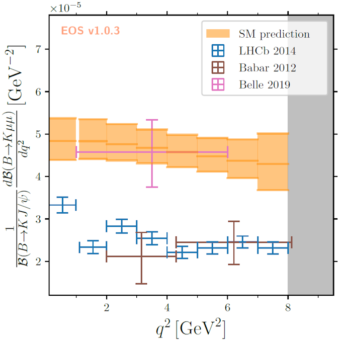
Figure 3: Tension between measurements and the SM prediction from Ref. [Gubernari:2020eftBIB] in the normalized differential branching ratio of \(B \to K \, \mu^+ \mu^-\).
Here \(q^2\) denotes the squared momentum transfer between the two hadrons.
There are several tensions between SM predictions and measurements in \(b\,\)-hadron decays observables.
Although their significance has not yet reached the 5-standard-deviation threshold in a single measurement — traditionally required for a new discovery — they remain intriguing and could indicate the presence of NP.
These tensions have been detected in both the FCCC transition \(b\to c\tau\bar\nu\) and the FCNC transition \(b\to s\mu^+\mu^-\).
Concerning the FCCC processes, the average of the measurements of the lepton flavour universality (LFU) ratios \(R_D\) and \(R_{D^*}\) exceed the SM prediction by 1.6σ and 2.6σ, respectively [HFLAV:2022pweBIB].
The combination of these two averages yields a tension of 3.3σ.
Concerning the FCNC processes, the LHCb and CMS measurements
[LHCb:2014cxeBIB,LHCb:2016yklBIB,LHCb:2021zwzBIB,CMS:2024syxBIB]
of the branching ratios and the angular observables in
\(B \to K^{(*)}\mu^+\mu^-\) and
\(B_s \to \phi\mu^+\mu^-\)
decays deviate from the SM predictions.
The significance of the \(b\to s\mu^+\mu^-\) tensions depends not only on the specific observable and bin considered, but also on the SM predictions used.
Due to the difficulties in estimating the relevant non-local MEs, there is no consensus in the theory community on the SM predictions for these observables.
Nevertheless, whether the tension is due to NP or underestimated theoretical uncertainties, it is clear that the current SM predictions cannot explain the experimental data.
For example, Ref. [Parrott:2022zteBIB] reports a 4.2σ tension for the \(B \to K\mu^+\mu^-\) branching fraction in the large recoil region. See also Figure 3.
These tensions together with others omitted here for brevity are commonly called the \(B\)anomalies.
Understanding the \(B\) anomalies is essential for advancements in the field.
In particular, the significance of the \(b\to s\mu^+\mu^-\) anomalies is high and has been confirmed by different measurements and/or experiments, and thus it is extremely unlikely that they are due to a mere statistical fluctuation.
The situation is made even more interesting by the fact that these anomalies form a coherent picture that suggests the existence of NP short-distance contributions (see, e.g., Ref. [Allanach:2023uxzBIB,Allanach:2024ozuBIB]).
Similarly, the \(b\to c\tau\bar\nu\) anomalies can be explained by introducing a new heavy mediator [Iguro:2024hykBIB].
In addition to the \(B\) anomalies, there is also a long puzzle in the determination of the CKM matrix elements \(|V_{ub}|\) and \(|V_{cb}|\), as the inclusive and exclusive determinations of these parameters differ by about 3σ [HFLAV:2022pweBIB].
Even though this tension is unlikely to be attributed to NP, it is important to resolve the \(|V_{ub}|-|V_{cb}|\) puzzle, since most predictions of flavour observables depend on these parameters.
In other words, the strength of the flavour constraints on NP critically depends on the precision of \(|V_{ub}|\) and \(|V_{cb}|\).
This puzzle can only be solved with an improvement of both the measurements and the calculations of the MEs in \(b\to u\tau\bar\nu\) and \(b\to c\tau\bar\nu\) decays.
Hadronic matrix elements calculations
I have shown in the previous paragraphs that precise theoretical predictions for MEs in \(b\,\)-hadron decays are indispensable for both NP searches and for the extraction of SM flavour parameters.
My research focuses on improving the precision of such MEs.
Especially for certain observables — e.g. the \(B \to K^* \, \mu^+ \mu^-\) differential branching ratio — the theoretical uncertainties are larger than the experimental ones.
Therefore, in order to make full use of the substantial investments and efforts made by the experimental collaborations dedicated to these measurements, advancements on the theoretical side are necessary.
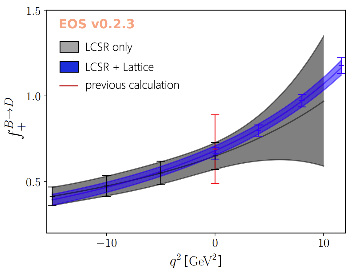
Figure 4: LCSR results for the \(f_+\) ME (or form factor) in \(B \to D\) processes from Ref. [Gubernari:2018wyiBIB].
Results are plotted as a function of the squared momentum transfer \(q^2\).
There are two QCD-based methods to compute MEs: lattice QCD (LQCD) and QCD sum rules.
On the one hand, LQCD is a first-principles method that allows the calculation of MEs.
The main advantage of LQCD computations is that their uncertainties can be systematically reduced, although they are time-consuming and resource-intensive.
On the other hand, QCD sum rules are based on an operator product expansion and the analytical properties of the correlation functions.
The evaluation of QCD sum rules requires knowledge of non-perturbative inputs, such as quark condensates or hadron distribution amplitudes, which are difficult to determine with high precision.
Nevertheless, QCD sum rules are extremely useful as they can currently provide insight into matrix elements where LQCD results are unavailable or limited.
Using the QCD light-cone sum rules (LCSRs) with \(B\)-meson distribution amplitudes, my collaborators and I have calculated the local MEs (i.e., the meson-to-meson form factors) in the most phenomenologically relevant \(B\) decays:
\(B \to \pi\),
\(B \to \rho\),
\(B \to K^{(*)}\),
\(B \to D^{(*)}\),
\(B_s \to \phi\).
\(B_s \to D_s^{(*)}\)
[Gubernari:2020eftBIB,Gubernari:2018wyiBIB,Bordone:2019gucBIB].
For the first time, our calculations included sub-leading power (or twist) corrections, which have a significant impact, amounting to a ~20% shift in the MEs results.
One of the MEs for the \(B \to D\) process is shown in Figure 4. As illustrated, LCSRs can be combined with lattice QCD results to determine the MEs across the entire kinematic region. In many cases, these two methods are complementary, as they are applicable in different regions of phase space. Their combination, therefore, enables more precise and reliable predictions.
Figure 5: Representation of a non-local contribution in \(B \to K\mu^+\mu^-\): the soft-gluon contribution to the charm loop.
In Ref. [Gubernari:2020eftBIB], we have recalculated the leading non-local MEs in \(B \to K^{(*)}\ell^+\ell^-\) decays (see Figure 5).
We have found that the power corrections to these non-local MEs — also known as soft-gluon contribution to the charm loop — are almost negligible.
This contradicts the results of Ref. [Khodjamirian:2010vfBIB], which found power corrections two orders of magnitude larger than ours.
Nevertheless, the origin of this difference is understood; it is mostly due to missing contributions in the previous calculation and updated hadronic inputs.
Another research direction I am pursuing is the derivation of unitarity bounds for MEs.
The unitarity bounds are model-independent constraints that can be used to further improve the precision of ME predictions.
In Ref. [Bordone:2019gucBIB], we have imposed these bounds and used heavy-quark effective theory to obtain very precise predictions for local MEs in \(B \to D^{(*)}\) and \(B_s \to D_s^{(*)}\) processes in the whole semileptonic region.
We have also derived the first unitarity bound for the non-local MEs in \(B \to K^{(*)}\ell^+\ell^-\) decays, providing unprecedented control over the systematic uncertainties of these objects [Gubernari:2020eftBIB].
I have further refined these bounds in Ref. [Gopal:2024mgbBIB], where I found an innovative method to systematically account for the effect specific branch cuts (i.e., subthreshold and anomalous cuts) that appear in b-hadron decays.
This method paves the way for a wide range of new ME analyses based solely on first principles, thereby minimising systematic uncertainties.
I have performed pioneering calculations of the local MEs in \(B \to D^{**}\ell \bar\nu\) decays
[Gubernari:2022hrqBIB,Gubernari:2023rfuBIB]
and the non-local MEs in \(\Lambda_b \to \Lambda\ell^+\ell^-\) decays [Feldmann:2023plvBIB].
These calculations are not only important because these MEs were previously unknown or poorly understood theoretically, but also because their completion required significant technical advancements in LCSRs.
In fact, both my numerical results and technical developments are widely used by other collaborations.
Predictions and phenomenological analyses for \(\,B\,\)-decays
Once the MEs are calculated, they can be used to predict observables in \(b\,\)-hadron decays.
These predictions are valuable because they can be compared with measurements to search for NP and extract the SM flavour parameters.
Performing these comparisons is often technically challenging, since there are usually several measurements and predictions for the same observable that need to be taken into account and combined to obtain the most accurate result.
In addition, the observables can be differential in several kinematic variables, such as the momentum transfer and the angles between the final state particles.
For this reason, complex statistical analyses are often required to perform comprehensive comparisons between theory and experiment.
To overcome these challenges, dedicated software tools have been developed, e.g. EOS, flavio, and HAMMER.
I am one of the senior developers of EOS, an open-source software project primarily written in C++ with a Python interface.
EOS can both predict flavour observables and perform Bayesian statistical analyses.
Using EOS, we have combined the available theoretical results (including our calculation of refs. [Gubernari:2018wyiBIB,Bordone:2019gucBIB]) to obtain precise predictions for \(B \to D^{(*)}\ell \bar\nu\) and \(B_s \to D_s^{(*)}\ell \bar\nu\) decays, such as the branching ratios, the angular observables, and the LFU ratios \(R_{D^{(*)}}\) and \(R_{D_s^{(*)}}\).
We have also provided an exclusive determination of \(|V_{cb}|\), which lowered the tension with the inclusive determination to 1.8σ, and hence alleviates the \(|V_{ub}|-|V_{cb}|\) puzzle.
In Ref. [Bordone:2020gaoBIB], we have used the results for the \(\bar{B}\to D^{(*)}\) and \(\bar{B}_s\to D_s^{(*)}\) local MEs to update the predictions for the hadronic decays \(\bar{B}_s^0\to D_s^{(*)+}\! \pi^-\) and \(\bar{B}^0\to D^{(*)+} K^-\).
The precision of our SM predictions uncovered a substantial discrepancy with respect to the experimental measurements at the level of 4.4σ.
We discuss the possible origins of this discrepancy in the article, which has triggered the interests of several research groups.
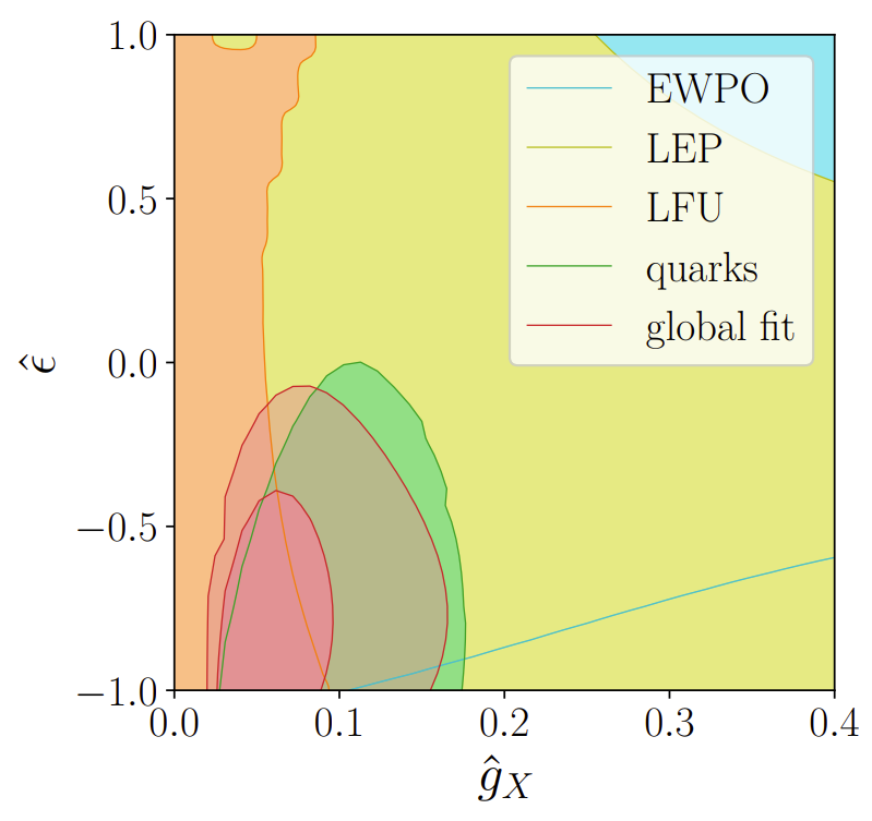
Figure 6: Parameter space of the malaphoric \(B_3 - L_2 Z'\) model. This model is characterised by the two parameters showed the plot, i.e. \(\hat{g}_X\) and \(\hat{\epsilon}\).
These parameters are zero in the SM.
We investigate the phenomenological consequences of the unitarity bound and the calculation of non-local MEs in \(B \to K^{(*)}\ell^+\ell^-\) and \(B_s \to \phi\ell^+\ell^-\) decays of Ref. [Gubernari:2020eftBIB] in Ref. [Gubernari:2022hxnBIB].
In this work we provide precise predictions for the differential branching ratios and angular observables in these decays.
We have also performed a global analysis of the \(b\to s\mu^+\mu^-\) transition.
We find a significant tension between the SM predictions and the experimental measurements for these decays, strengthening the \(b\to s\mu^+\mu^-\) anomalies.
At the University of Cambridge, I am currently working with prof. B. Allanach on the development NP models that can explain the \(b\to s\mu^+\mu^-\) anomalies [Allanach:2024ozuBIB].
This research is important to understand whether there is a viable NP explanation for the anomalies and to guide the experimental searches for NP at the LHC and future colliders.
If such NP explanation does not exist, the anomalies would be a sign of underestimated theoretical oe experimental uncertainties, which would require a revision of the SM predictions and measurements for these decays.
It is important to note that the \(b\to s\mu^+\mu^-\) anomalies form a coherent picture, as they can be explained by certain NP models, such as leptoquarks or \(Z'\) bosons.
For instance, in Ref. [Allanach:2024ozuBIB] we show that the "malaphoric" \(Z'\) model explains the current data better than the SM. This can be seen in Figure 6.
These findings highlight the need for further theoretical and experimental investigations to conclusively determine the origin of the \(b\to s\mu^+\mu^-\) anomalies. Future measurements at the LHC and upcoming collider experiments, along with refined theoretical calculations, will be crucial in distinguishing between potential new physics explanations and underestimated uncertainties within the SM.
References
N. Gubernari, D. van Dyk, J. Virto,
Non-local matrix elements in \(B_{(s)}\to \{K^{(*)},\phi\}\ell^+\ell^-\),
JHEP 02 2021 088
[2011.09813].
Y.S. Amhis, others,
Averages of b-hadron, c-hadron, and \(\tau\)-lepton properties as of 2021,
Phys. Rev. D 107 2023 052008
[2206.07501].
R. Aaij, others,
Differential branching fractions and isospin asymmetries of \(B \to K^{(*)} \mu^+ \mu^-\) decays,
JHEP 06 2014 133
[1403.8044].
R. Aaij, others,
Measurements of the S-wave fraction in \(B^{0}\rightarrow K^{+}\pi^{-}\mu^{+}\mu^{-}\) decays and the \(B^{0}\rightarrow K^{\ast}(892)^{0}\mu^{+}\mu^{-}\) differential branching fraction,
JHEP 11 2016 047
[1606.04731].
R. Aaij, others,
Branching Fraction Measurements of the Rare \(B^0_s\rightarrow\phi\mu^+\mu^-\) and \(B^0_s\rightarrow f_2^\prime(1525)\mu^+\mu^-\)- Decays,
Phys. Rev. Lett. 127 2021 151801
[2105.14007].
A. Hayrapetyan, others,
Test of lepton flavor universality in B\(^{\pm}\)\(\to\) K\(^{\pm}\mu^+\mu^-\) and B\(^{\pm}\)\(\to\) K\(^{\pm}\)e\(^+\)e\(^-\) decays in proton-proton collisions at \(\sqrt{s}\) = 13 TeV,
Rept. Prog. Phys. 87 2024 077802
[2401.07090].
W.G. Parrott, C. Bouchard, C.T.H. Davies,
Standard Model predictions for B\(\to\)K\(\ell\)+\(\ell\)-, B\(\to\)K\(\ell\)1-\(\ell\)2+ and B\(\to\)K\(\nu\)\(\nu\) using form factors from Nf=2+1+1 lattice QCD,
Phys. Rev. D 107 2023 014511
[2207.13371].
B. Allanach, A. Mullin,
Plan B: new Z' models for b \(\to\) s\(\ell\)\(^{+}\)\(\ell\)\(^{−}\) anomalies,
JHEP 09 2023 173
[2306.08669].
B. Allanach, N. Gubernari,
Malaphoric \(Z'\) models for \(b \rightarrow s \ell^+ \ell^-\) anomalies,
Eur. Phys. J. C 85 2025 2
[2409.06804].
S. Iguro, T. Kitahara, R. Watanabe,
Global fit to b\(\to\)c\(\tau\)\(\nu\) anomalies as of Spring 2024,
Phys. Rev. D 110 2024 075005
[2405.06062].
N. Gubernari, A. Kokulu, D. van Dyk,
\(B\to P\) and \(B\to V\) Form Factors from \(B\)-Meson Light-Cone Sum Rules beyond Leading Twist,
JHEP 01 2019 150
[1811.00983].
M. Bordone, N. Gubernari, D. van Dyk, M. Jung,
Heavy-Quark expansion for \({{\bar{B}}_s\rightarrow D^{(*)}_s}\) form factors and unitarity bounds beyond the \({SU(3)_F}\) limit,
Eur. Phys. J. C 80 2020 347
[1912.09335].
A. Khodjamirian, T. Mannel, A.A. Pivovarov, Y.-. Wang,
Charm-loop effect in \(B \to K^{(*)} \ell^{+} \ell^{-}\) and \(B\to K^*\gamma\),
JHEP 09 2010 089
[1006.4945].
A. Gopal, N. Gubernari,
Unitarity bounds with subthreshold and anomalous cuts for b-hadron decays,
Phys. Rev. D 111 2025 L031501
[2412.04388].
N. Gubernari, A. Khodjamirian, R. Mandal, T. Mannel,
\(B \to D_1 (2420)\) and \(B \to D_1^\prime (2430)\) form factors from QCD light-cone sum rules,
JHEP 05 2022 029
[2203.08493].
N. Gubernari, A. Khodjamirian, R. Mandal, T. Mannel,
\( B\to {D}_0^{\ast } \) and \( {B}_s\to {D}_{s0}^{\ast } \) form factors from QCD light-cone sum rules,
JHEP 12 2023 015
[2309.10165].
T. Feldmann, N. Gubernari,
Non-factorisable contributions of strong-penguin operators in \(\Lambda_b \to \Lambda \ell^+\ell^-\) decays,
JHEP 03 2024 152
[2312.14146].
M. Bordone, N. Gubernari, T. Huber, M. Jung, D. van Dyk,
A puzzle in \(\bar{B}_{(s)}^0 \to D_{(s)}^{(*)+} \lbrace \pi^-, K^-\rbrace\) decays and extraction of the \(f_s/f_d\) fragmentation fraction,
Eur. Phys. J. C 80 2020 951
[2007.10338].
N. Gubernari, M. Reboud, D. van Dyk, J. Virto,
Improved theory predictions and global analysis of exclusive \(b \to s\mu^+\mu^-\) processes,
JHEP 09 2022 133
[2206.03797].
Outreach
This section is intended for people who have no prior knowledge of quantum physics and particle physics but would like to explore the subject.
In the following paragraphs, I provide a concise and accessible introduction to these fields, starting with key concepts such as the structure of matter and its building blocks.
I then take a closer look at the structure of the atom and explain what antimatter is.
Next, I discuss the importance of particle accelerators and the role of (quantum) particle collisions in advancing our understanding of the universe.
Finally, I introduce my field of research, flavour physics, highlighting its purpose and scientific relevance.
Please contact me if you have any comments, questions, or suggestions about this section.
Contents
Physics: The study of nature
Curiosity is one of the defining characteristics of human beings, driving us to ask questions, seek answers, and explore the mysteries of the universe.
It is this profound curiosity that motivates our thirst for knowledge, fuels our scientific discoveries, and shapes the course of our history.
In this relentless quest, curiosity has led us to ponder fundamental issues such as: What are we made of? How did our universe originate? What are space and time?
Physics aims to answer these questions through the systematic study of nature.
Among the different branches of physics, I am principally interested in particle physics.
The ultimate goal of this field of research is to understand the fundamental constituents of matter and the forces that govern their behaviour.
What are we made of?
Every day we see and touch hundreds of objects.
The variety of shapes, colours, and sizes we observe is astonishing.
Even more amazing is the fact that everything is made up of only 17 different types of fundamental — i.e. indivisible — particles.
These are the basic building blocks of matter.
But let us take things one step at a time, starting with the atoms.
The idea that matter is made up of basic building blocks goes back a long way.
It was first proposed by the ancient Greek philosophers Leucippus and Democritus of Abdera in the 5th century BC.
That is why the word atom comes from the ancient Greek word atomos, meaning indivisible.
However, these were mere speculations and the modern scientific understanding of the atom began to emerge in the 19th century.
In 1803, John Dalton proposed his atomic theory, supported by strong experimental evidence.
According to this theory, matter is made up of tiny, indivisible particles (the atoms).
He also suggested that not all atoms are the same, but that there are various types with distinct properties.
To date, 118 different types of atoms (or elements) have been identified.
This is likely close to the maximum number of elements possible, due to nuclear stability limits.
The most common elements on Earth include oxygen, aluminium and iron.
Atoms are extremely small compared to the objects we usually deal with in our everyday lives.
The typical diameter of an atom is about 0.1 nanometres (one ten-millionth of a millimetre).
To give you an idea of how small atoms are, a grain of salt contains about a quintillion atoms, or if you prefer, a million million million (=1,000,000,000,000,000,000) atoms.
Please take this information with a grain of salt.
Atoms can combine to form molecules through chemical bonds.
Molecules, in turn, assemble into complex structures such as cells – the basic units of life.
Within cells, intricate processes take place to carry out the functions necessary for life.
In the case of humans, trillions of cells, each with specific roles and functions, come together to form tissues, organs, and ultimately an entire organism.
The discovery of the atom was undoubtedly one of the greatest achievements in human history.
Thanks to this discovery, we can now diagnose diseases, generate energy and develop new materials for various applications.
However, we now know that atoms are not the fundamental building blocks of matter.
In other words, they are made up of other particles that, according to our current knowledge, are fundamental.
Hence, to get the ultimate answer to the question "What are we made of?", we have to answer the question "What are atoms made of?".
But how can we find out what is inside something so small?
Aside: The structure of matter (and antimatter)
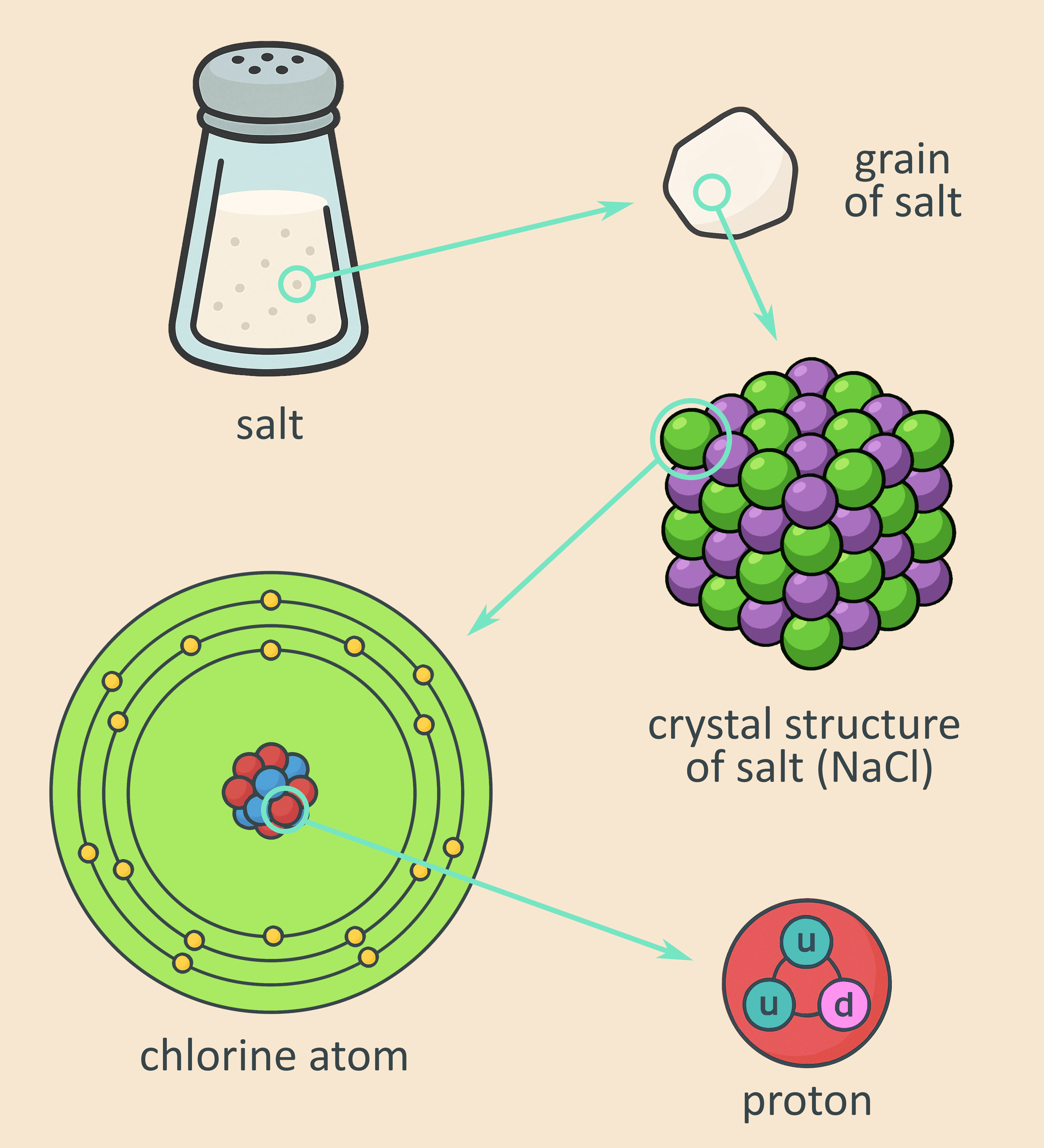
This image illustrates the structure of matter from macroscopic to subatomic levels, starting with salt in a shaker, zooming into a grain of salt, then into its crystal structure (sodium chloride, NaCl), showing individual chlorine atoms, and finally down to a proton composed of three quarks (up and down types).
Note that the image is not entirely accurate. As discussed in the text, the nucleus is much smaller than the atom itself, and quarks are considered point-like particles with no measurable size. Additionally, electrons do not orbit the nucleus in fixed paths; instead, they move within a diffuse region called a "cloud of probability," which represents where they are likely to be found at any given time.
Before continuing, let me clarify some concepts that are fundamental to understanding the following sections.
Every atom is made up of a nucleus and electrons orbiting around it, like a miniature solar system. (This is a simplified picture, but sufficient for our purposes.)
The nucleus contains almost all the mass of the atom, about 99.9%, while the electrons, being much lighter, contribute negligibly to the total mass, i.e. less than 0.01%.
The nucleus itself is about 10,000 times smaller than the atom as a whole.
To put this in perspective, if the nucleus were the size of a football (soccer ball), the atom would be the size of a football stadium.
The nucleus is made up of protons and neutrons. Protons have a positive charge, while neutrons have no charge.
Since the atom is electrically neutral, the number of protons is equal to the number of electrons.
The only thing that distinguishes one element from another is the number of protons in its nucleus.
For example, hydrogen has one proton, helium has two, and so on.
However, the number of elements is finite, as I mentioned earlier.
This is due to the fact that nuclei with many protons and neutrons are unstable and decay into lighter nuclei.
It is important to emphasize that, based on our current understanding, protons and neutrons are not fundamental particles. Instead, they are composed of even smaller, point-like constituents known as quarks. (See the figure on the left.)
In contrast, electrons are considered truly fundamental particles.
Let me mention something that a physicist might consider trivial, but not everyone is familiar with.
Whenever we touch an object, like a table, what happens at the microscopic level is that the electrons in the atoms of our fingertips repel the electrons in the atoms of the table.
This is due to the electromagnetic force, which implies that like-charged particles (such as electrons) repel each other.
As a result, we never actually "touch" anything in the sense of direct contact at the atomic level. Instead, it is the electromagnetic force between the electrons that we perceive as the sensation of touch.
Furthermore, all fundamental particles are considered to be point-like, that is they have no volume.
Therefore, there is never any direct contact between particles, but only interactions through the fundamental forces (electromagnetic, weak, strong, and gravitational).
Since fundamental particles have no volume, the total volume of all fundamental particles in the universe is exactly zero. In other words, everything we see around us is made of particles that, taken together, occupy no space at all – a conclusion that is both counter-intuitive and astonishing.
Another important concept to clarify is that of antimatter.
Antimatter is like a mirror image of matter. For every type of particle in matter, there is a corresponding antiparticle in antimatter. For example, the antiparticle of an electron (negatively charged particle) is called a positron (which has a positive charge).
When matter and antimatter come together, they annihilate each other in a burst of pure energy.
This energy release is extremely powerful.
According to Einstein's famous formula \(E=mc^2\), the energy released is equal to the mass of the particles multiplied by the speed of light squared.
For instance, if just a few grains of ordinary salt were to meet an equal amount of antimatter salt, they would release an amount of energy equivalent to that released by the Little Boy bomb dropped on Hiroshima in 1945. (Please take this information with a grain of salt.)
This comparison may sound almost unbelievable and it highlights just how astonishingly powerful matter-antimatter annihilation is.
Fortunately, our universe is made almost entirely of matter, while only a tiny amount of antimatter is produced in very energetic processes.
So rest assured: the next time you put salt on your pasta, you are not at risk of triggering a nuclear explosion.
One might naturally expect antimatter and matter to be equally abundant in the universe, and our current theories largely suggest this.
But what we observe is different.
The fact that the universe is predominantly composed of matter remains one of the greatest unsolved mysteries in contemporary physics.
The dawn of particle physics
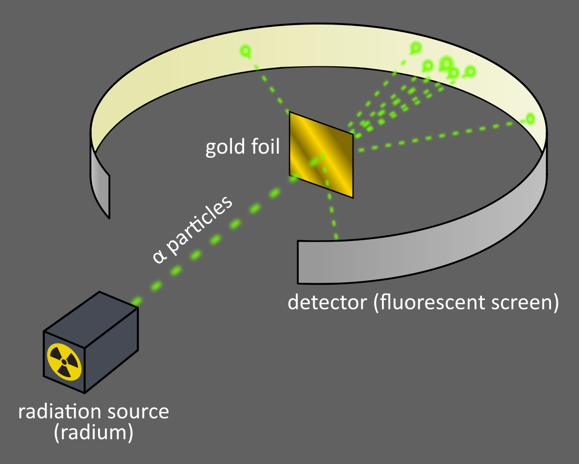
In Rutherford's gold foil experiment, most \(\alpha\) particles passed through a thin sheet of gold, but some deflected sharply or bounced back. This revealed that atoms are mostly empty space, with nearly all their mass and positive charge concentrated in a tiny central nucleus—replacing earlier models of the atom.
I was tempted to call this section “The story of physicists and their passion for smashing particles together.” Unfortunately, that title was too long, so I chose a shorter one instead.
The story of particle physics begins at the end of the 19th century, when Thomson discovered the electron at the Cavendish Laboratory of Cambridge University in 1897.
A few years later, Geiger and Marsden, under the supervision of Rutherford, carried out a series of experiments to clarify the structure of the atom.
The experiment that went down in history consisted of firing positively charged particles — called \(\alpha\) particles, which we now know to be helium nuclei — at a gold foil.
Geiger and Marsden observed to their amazement that about one out of every ten thousand \(\alpha\) particles was reflected, i.e. deflected at an angle greater than 90°, while the rest passed through the foil or underwent slight deflection (see figures).
The astonishment arose from the fact that the atomic model of the time proposed by Thomson himself did not predict such a result.
Indeed, in Thomson's model, atoms looked like a "plum pudding", with the positive charge evenly distributed throughout the atom and the negatively charged electrons embedded in it.
According to this model, most of the \(\alpha\) particles should have passed straight through the foil with very little or no deflection, as they encountered very few obstacles.
Rutherford himself famously explained this result by saying, "It was as if you had fired a 15-inch shell at a piece of tissue paper and it had come back and hit you".
To explain the experimental results, Rutherford proposed a new atomic model.
In this new model the positive charge is concentrated in a compact nucleus at the centre of the atom, while the electrons revolve around the nucleus itself (as explained in the previous section). For this reason, the Rutherford model is also called the planetary model.
This model laid the foundation for the later quantum model of the atom proposed by Bohr, which remains a useful approximation, even though modern quantum mechanics provides a more accurate description.
In Rutherford's atomic model, most \(\alpha\) particles passed through the atom undeflected, showing that atoms are mostly empty space. A small fraction deflected at sharp angles or bounced back, demonstrating the presence of a tiny, dense, positively charged nucleus at the center
Geiger and Marsden's experiment illustrates one of the reasons why colliding particles can be useful.
By either shooting particles at a fixed target or colliding them with each other, we can probe both their effective "shape" and whether they have an internal substructure.
(Here, "shape" refers to the geometry of the forces through which the particles interact. In the experiment described, it is the electromagnetic potential of the gold nucleus.)
There is no other way to understand what is inside an atom, or even more so, what happens inside the nucleus of an atom, as it is impossible to observe such phenomena with any optical microscope.
In fact, an atom is tens of thousands of times smaller than the wavelength of light visible to the human eye.
Such experiments can therefore be seen as a natural evolution of the idea of the optical microscope.
The concept of probing the shape of particles and their internal structure through collisions is the basis of particle physics.
Hence, I will try to further clarify it using a simple example.
Imagine opening a garage door.
You are outside the garage and you want to know what is inside.
However, the garage is dark and you cannot see anything.
You can also smell gas, so you do not want to enter the garage for fear of being poisoned.
Fortunately, you have just come from a fantastic tennis match (you won 6-2 6-1) and you have some tennis balls with you.
You have an idea.
You throw the tennis balls inside the garage and observe how they bounce back.
From the way the tennis balls bounce back and the time they take to do so, you can immediately understand how full the garage is.
By analysing the bounces more carefully, you can also understand the shape of the objects inside the garage.
Have I convinced you that colliding particles is a good way to study their properties?
The advent of particle accelerators
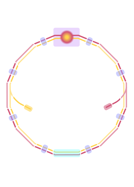
Diagram of a particle collider known as a synchrotron.
Electrons and positrons are injected into the ring, accelerated to very high speeds, and guided by powerful magnets. They travel in opposite directions until they collide at the detector.
The first particle accelerators were built in the late 1920s, although particle physics developed mainly after the Second World War.
The purpose of these machines is to create beams of particles, accelerate them to speeds close to the speed of light, and make them collide with each other.
(The speed of light is about 3·108m/s, or more than a billion kilometres per hour.)
The particles most commonly used are protons, electrons, antiprotons and positrons, although heavy metal nuclei are also sometimes used.
Some accelerators collide beams of the same particles (e.g. electron-electron), while others collide two beams of different particles (e.g. electron-positron, electron-proton).
Most modern accelerators are synchrotrons.
The Large Hadron Collider (LHC) at CERN in Switzerland, better known as the LHC, is the world's largest and most powerful accelerator, a proton-proton synchrotron.
The LHC is one of the most impressive feats ever achieved by mankind. It cost around €4.75 billion to build (not including the cost of digging the 27-kilometre tunnel that houses the accelerator and the four caverns that house the various experiments) and requires an additional €1 billion a year to operate.
Synchrotrons have a roughly circular shape (in practice, polygonal) and consist of two parallel pipes, each with a diameter of several tens of centimetres, through which particle beams travel. The particle beams in the two different pipes travel in opposite directions (see figure).
The pipes are kept under vacuum so that the beams can travel without interference from air molecules.
In a synchrotron, beams of particles are accelerated along the two pipes by alternating electric fields, while magnetic fields guide and concentrate the beams, keeping them on a circular trajectory and tightly focused.
The maximum (kinetic) energy that a synchrotron can reach is determined mainly by two factors.
The first is the type of particle being accelerated. The heavier the particle, the greater its energy.
The second is the circumference of the synchrotron.
With each revolution, a particle gradually loses energy. In fact, when a charged particle's path is curved, it emits radiation, causing energy loss. This radiation is called synchrotron radiation.
For this reason, particles cannot be accelerated indefinitely: at a certain point, the energy provided by the electric fields at each revolution equals the energy lost to synchrotron radiation.
Since synchrotron radiation decreases for larger radii, synchrotrons with greater circumference can reach higher energies.
This explains why we need an accelerator 27 kilometres long like the LHC, and why we will need an even larger one if we want to reach higher energies.
Quantum collisions
Particle accelerators are much more than just sophisticated microscopes for studying the shapes of potentials and the possible substructure of particles.
To understand this, we first need to look at the difference between classical and quantum collisions.
Let us consider, for example, a billiard table.
Classical mechanics tells us that when billiard balls collide, they scatter in different directions.
If we know their directions and speeds before the collision, we can calculate their directions and speeds afterwards.
One could also increase the speed of the balls disproportionately, causing them to jump off the table or even break on impact, but no fundamentally new phenomena would occur.
Unlike classical collisions where objects merely bounce off each other, high-energy quantum collisions can transform energy into entirely new particles, revealing the fundamental building blocks of matter. Thanks to Einstein's equation \(E=mc^2\), the mass of the particles created can be far greater than the mass of the particles that collided.
That seems fairly intuitive, doesn't it? But in quantum (relativistic) mechanics, collisions can have very different outcomes.
As I mentioned above, this is Einstein's famous formula: \(E=mc^2\).
This formula implies that mass and energy are equivalent — in other words, they are two sides of the same coin.
Hence, mass can be converted into energy and vice versa.
The case of matter-antimatter annihilation is an example of the conversion of mass into energy.
In high-energy particle collisions, the reverse happens: energy can be converted into mass.
The mass-energy equivalence, which may seem strange at first, has surprising consequences.
The energy released in a collision generates new particles, sometimes very different from the ones that originally collided.
For instance, by colliding two electrons, it is possible to create any particle in the universe, provided its mass is less than or equal to the available collision energy.
Thus, in the quantum world, the collision of two billiard balls at sufficient speed could result in the formation of entirely new and unexpected objects, such as a rugby ball, a cake, or even a house.
Strange, isn't it?
Let me point out something about this example.
While it's true that in theory, particles and billiard balls at sufficient energy levels could potentially form macroscopic objects through various interactions and combinations, in practice, this doesn't occur for two main reasons.
First, it is not realistically possible to achieve the enormous energies required to trigger such phenomena.
Second, the likelihood of collision products arranging themselves into recognizable macroscopic objects, like rugby balls or houses, is astronomically small, due to the complexity of such arrangements and the random nature of quantum processes.
Nevertheless, quantum effects do occur and are observable in collisions between subatomic particles.
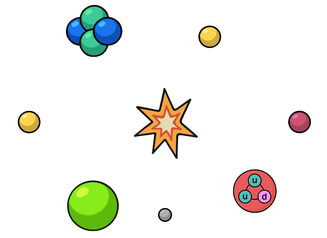
The 17 fundamental particles of the Standard Model: six quarks, six leptons, four force carrier particles (photon, gluon, W and Z bosons), and the Higgs boson, which gives particles mass.
Antimatter counterparts of these particles are not shown explicitly.
By colliding electrons and/or protons in particle accelerators, physicists have been able to create the fundamental particles (or what we currently believe to be fundamental) that constitute the entire visible universe.
To date, 17 (types of) fundamental particles have been identified, neatly summarized in a theory called the Standard Model and shown in the image.
The Standard Model was first formulated in the late 1960s and, over the following decades, was refined and expanded into the framework we know today. Despite the passage of time, it continues to describe with remarkable accuracy the behaviour of the fundamental particles and their interactions.
These 17 types of particles fall into families with different roles. Quarks come in six types—up, down, charm, strange, truth, and beauty.
Protons and neutrons, the heart of every atom, are made from up and down quarks, while the heavier quarks appear only in high-energy environments such as cosmic rays or particle accelerators.
Alongside them are the leptons: the well-known electron, familiar from atoms and electricity, its heavier "brothers" the muon and tau, and three types of elusive neutrinos (electron, muon, and tau neutrinos) that pass through us with hardly any interaction.
Forces are carried by their own particles: the photon, responsible for light and electromagnetism; the gluon, which glues quarks together inside protons and neutrons; and the W and Z bosons, which govern the weak force that drives certain radioactive decays and plays a key role in nuclear fusion inside stars. Completing the picture is the Higgs boson, linked to the Higgs field that gives mass to the other fundamental particles.
Gravity, however, remains the great exception: we expect it to be carried by a hypothetical particle called the graviton, but this has not yet been observed, and gravity is still not explained by the Standard Model. This is one of the biggest open questions in physics.
In practice, almost all the matter we encounter every day is made of just up and down quarks (in protons and neutrons) and electrons.
The rest of the particles exist only briefly in the extreme environments of the universe or in the detectors of modern accelerators.
I find it astonishing that just a few fundamental particles can give rise to the entire richness of the universe we see and know. They combine in countless ways, like letters forming words, to form atoms, molecules, stars, planets, and ultimately life itself.
I hope that I have convinced you that colliding subatomic particles is far more fascinating than it might first appear.
For instance, every collision at the LHC between two protons produces thousands of new particles.
This illustrates the immense complexity of the field: at the LHC, around 600 million collisions occur every second: a challenge for experimental physicists, who must detect and analyze them, and for theorists like me, who work to predict and interpret their outcomes.
To put it in perspective: in just one second, the LHC produces more data than you could fit on thousands of DVDs. This gives us a truly astonishing window into the fundamental workings of the universe.
We pursue this by comparing precise experimental measurements with theoretical predictions from the Standard Model. If experiment and theory agree, it confirms that the Standard Model still provides an accurate description of fundamental interactions, with the important exception of gravity, which is not yet included. If they disagree, it signals that our theory is incomplete and must be extended or modified.
This effort explains the need for ever more powerful particle accelerators. By reaching higher energies, we can produce new particles that have never been observed before, potentially going beyond the Standard Model.
The discovery of new particles is not an end in itself but a crucial step toward a deeper understanding of nature. Each new particle provides a missing piece of the puzzle, helping us explore profound open questions: why is there more matter than antimatter in the universe? What is the nature of dark matter? How can gravity be unified with the other fundamental forces?
In this sense, particle physics is not only about smashing particles together but about pushing the boundaries of human knowledge, striving to uncover the ultimate laws of the universe.
Flavourful particles
My research focuses on flavour physics.
The name comes from the fact that the six different types of quarks are called flavours. Flavour physics explores in detail how quarks interact and decay. Its goal, once again, is to test the Standard Model. But rather than searching for new particles at ever higher energies, flavour physics performs precision tests.
In other words, by comparing experimental measurements of quark decays with precise theoretical predictions, we may uncover evidence for new particles indirectly. If the measurements differ from our calculations, it suggests the existence of new forces — and possibly new particles — beyond those we know today.
I focus particularly on the study of the beauty (or bottom) quark, one of the heaviest quarks and therefore especially valuable for testing the limits of the Standard Model. Its decays provide a sensitive window into possible new physics hiding beyond our current theories.
If you would like to dive deeper into this topic, feel free to explore the Research section – it goes into more technical detail.
I hope you enjoyed reading this introduction. If you have any comments or questions, please don't hesitate to contact me!
About me
Lorem ipsum dolor sit amet, consectetur et adipiscing elit. Praesent eleifend dignissim arcu, at eleifend sapien imperdiet ac. Aliquam erat volutpat. Praesent urna nisi, fringila lorem et vehicula lacinia quam. Integer sollicitudin mauris nec lorem luctus ultrices. Aliquam libero et malesuada fames ac ante ipsum primis in faucibus. Cras viverra ligula sit amet ex mollis mattis lorem ipsum dolor sit amet.